Shredding Cabbage I: The Uniform Spacing Model
Two Ways to Shred a Cabbage
I came up with the following question when I was cooking and shredding a large piece of cabbage by hand: given a piece of cabbage, if I randomly shred it into \(n\) pieces, what is the expected size of the largest piece? In general, what is the expected size of the \(i\)-th largest piece?
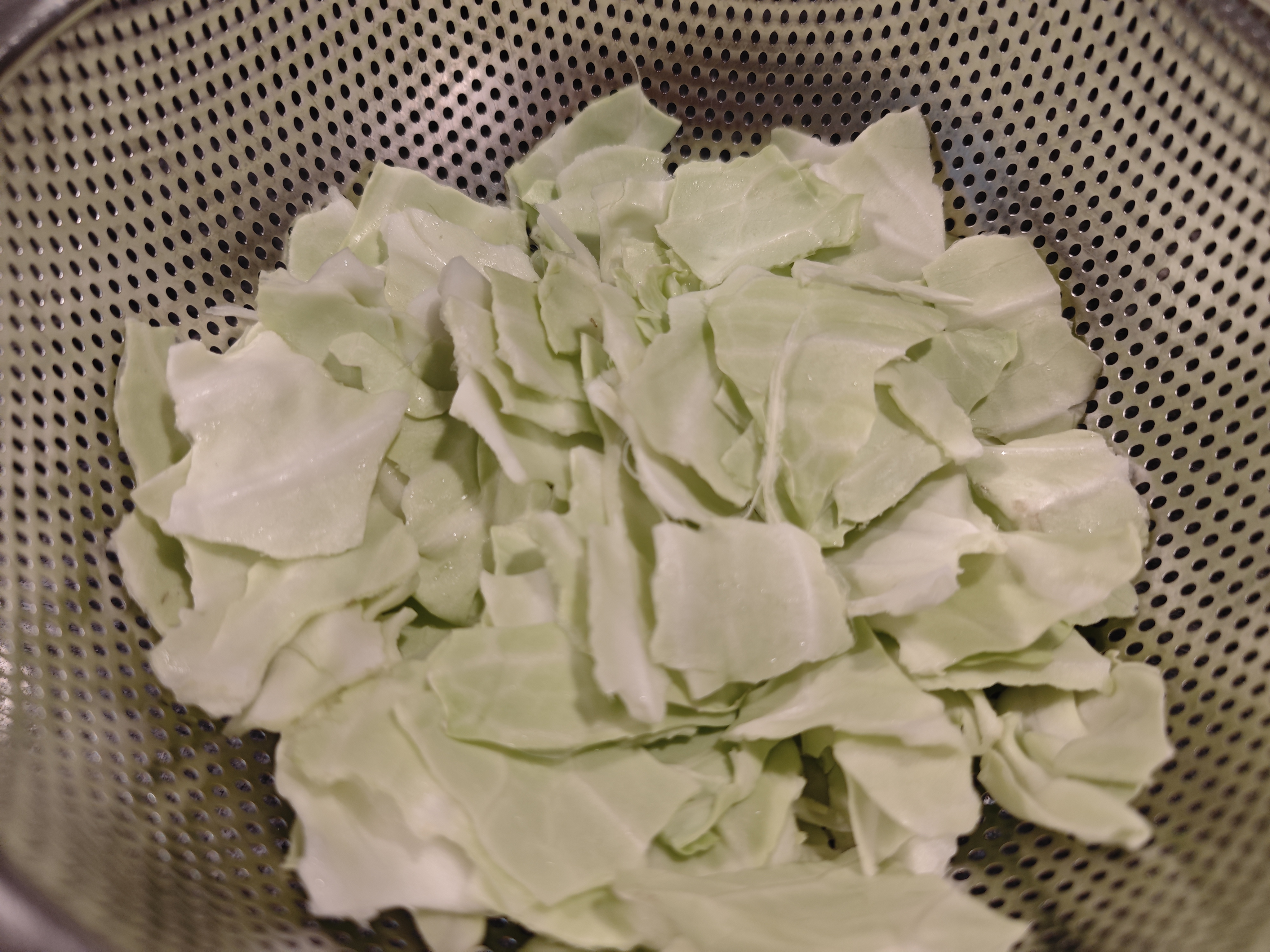
There are two natural ways to model “randomly” shredding. Formally, given an interval \([0,1]\) (the full piece of cabbage),
- Model 1: sample \(n-1\) points independently and uniformly at random from \([0,1]\). These points divide the interval into \(n\) pieces. Equivalently, this process can be interpreted as: in each step, take a piece with probability proportional to its size, and split at a uniformly random point within the piece.
- Model 2: Repeat the following \(n-1\) times to obtain \(n\) pieces: pick the longest piece (tie-breaking is not important) and split at a uniformly random point within the piece.
It turns out that both models have been studied in the literature.
Model 1 is known as the uniform (spacing) model (U-model), and appears at least as early as Problems 666–667 in Whitworth (1897).
Model 2 is known as the Kakutani model (K-model). It was first proposed by Shizuo Kakutani and later formally studied in van Zwet (1978).
In both models, we are interested in the order statistics of the pieces. Let \[ S_{[1]} \geq S_{[2]}\geq\cdots\geq S_{[n]} \] denote the lengths of the \(n\) pieces, sorted from longest to shortest. The main question is:
What is the expected length \(\mathbb E[S_{[i]}]\) of the \(i\)-th longest piece?
This post will focus on the U-model. In future posts I will discuss the same problem for the K-model, and some other related problems for both models.
Expected Lengths in the U-Model
The U-model has a long history. The expected lengths of the pieces have been studied in Whitworth (1897), Fisher (1929), Stevens (1939), Barton and David (1956), and Holst (1980). This post follows the proof strategy given by Holst (1980).
Theorem 1: let \(S_{[i]}\) be the length of the \(i\)-th longest piece obtained by dividing \([0,1]\) at \(n-1\) independent uniformly random points. Then \[ \mathbb E[S_{[i]}]=\frac{1}{n}\sum_{j=i}^n\frac{1}{j}, \text{ for }i=1,2,\ldots,n ~. \] In particular, the expected length of the longest piece is \(\mathbb E[S_{[1]}]=\frac{H_n}{n}\), where \(H_n\) is the \(n\)-th harmonic number; the expected length of the shortest piece is \(\mathbb E[S_{[n]}]=\frac{1}{n^2}\).
The following table demonstrates the numerical results for \(n=1,2,3,4,5\).
| \(n\) | \(\mathbb E[S_{[1]}]\) | \(\mathbb E[S_{[2]}]\) | \(\mathbb E[S_{[3]}]\) | \(\mathbb E[S_{[4]}]\) | \(\mathbb E[S_{[5]}]\) |
|---|---|---|---|---|---|
| 1 | 1.0000 | ||||
| 2 | 0.7500 | 0.2500 | |||
| 3 | 0.6111 | 0.2778 | 0.1111 | ||
| 4 | 0.5208 | 0.2708 | 0.1458 | 0.0625 | |
| 5 | 0.4567 | 0.2567 | 0.1567 | 0.0900 | 0.0400 |
Relation to Exponential Random Variables
The first step of the proof is to show that the distribution of the lengths of the pieces (from left to right) is related to independent exponential random variables.
Let \(E_1,E_2,\ldots,E_n\) denote \(n\) independent exponential random variables with mean \(1\). For each \(i\in[n]\), the density of \(E_i\) is \(f_{E_i}(x) = e^{-x}, x\geq 0\), and \(\Pr[E_i>x] = e^{-x}\). Let \(T_n = \sum_{i=1}^n E_i\).
Let \[ 0=U_{(0)}<U_{(1)}<\cdots<U_{(n-1)}<U_{(n)}=1 \] denote the endpoints of the pieces, where \(U_{(1)},\ldots,U_{(n-1)}\) are obtained by sorting the \(n-1\) random splitting points. Let \[ S_j=U_{(j)}-U_{(j-1)},\qquad 1\leq j\leq n \] denote the lengths of the pieces (from left to right, without sorting).
Since the splitting points are sampled from a continuous distribution, with probability \(1\) they are distinct and lie strictly inside \((0,1)\). Thus, we assume all piece lengths are positive. We will nevertheless use the corresponding closed regions for convenience. Their boundaries have \((n-1)\)-dimensional volume \(0\), so including or excluding the boundaries does not affect any density, probability, or integral below.
Lemma 2: the distribution of \((S_1,\ldots,S_n)\) satisfies \[ (S_1,\ldots,S_n)\sim \left(\frac{E_1}{T_n},\ldots,\frac{E_n}{T_n}\right) ~. \]
Proof: both sides can be viewed as an \(n\)-tuple with non-negative entries that sum to \(1\), i.e., once the first \(n-1\) entries are given, the last entry is automatically fixed. So we focus on the first \(n-1\) entries, and the proof reduces to the following: prove that \((S_1,\ldots,S_{n-1})\) and \(\left(\dfrac{E_1}{T_n},\ldots,\dfrac{E_{n-1}}{T_n}\right)\) are identically distributed over the \((n-1)\)-dimensional region \[ \left\{(x_1,\ldots,x_{n-1}): x_i\geq 0,\forall i\in[n-1]; \sum_{i=1}^{n-1}x_i \leq 1\right\} ~. \] This region has volume \(\frac{1}{(n-1)!}\), and in fact we will show that both tuples have constant density \((n-1)!\).
Left Side:
The \(n-1\) splitting points are independent and uniformly distributed over \([0,1]\), so their joint density is \(1\) over the unit cube \([0,1]^{n-1}\). Each ordered tuple \((U_{(1)},\ldots,U_{(n-1)})\) corresponds to exactly \((n-1)!\) possible configurations before sorting. Therefore, \((U_{(1)},\ldots,U_{(n-1)})\) is uniformly distributed over the region \[ \{ (u_1,\ldots,u_{n-1}): 0<u_1<u_2<\cdots<u_{n-1}<1\} \] with constant density \((n-1)!\).
There is a one-to-one correspondence between the ordered splitting points and the piece lengths on their respective domains:
- \(S_i = U_{(i)}-U_{(i-1)}\), for all \(i\in[n]\);
- \(U_{(i)} = \sum_{j=1}^i S_j\), for all \(i\in[n-1]\).
The transformation from the ordered splitting points to the piece lengths is linear and can be represented in matrix form: \[ (S_1,\ldots,S_{n-1}) = (U_{(1)},\ldots,U_{(n-1)}) \begin{pmatrix} 1 & -1 & 0 & \cdots & 0\\ 0 & 1 & -1 & \cdots & 0\\ 0 & 0 & 1 & \ddots & \vdots\\ \vdots & \vdots & \ddots & \ddots & -1\\ 0 & 0 & \cdots & 0 & 1 \end{pmatrix} ~. \] The matrix is upper triangular with all diagonal entries equal to \(1\), so its determinant is \(1\). Therefore, the transformation preserves volume, so we can conclude that \((S_1,\ldots,S_{n-1})\) has the same constant density \((n-1)!\) over the region \[ \left\{(x_1,\ldots,x_{n-1}): x_i\geq 0,\forall i\in[n-1]; \sum_{i=1}^{n-1}x_i \leq 1\right\} ~. \]
Right Side:
Consider calculating the density of \(\left(\dfrac{E_1}{T_n},\ldots,\dfrac{E_{n-1}}{T_n}\right)\) from the density of \((E_1,\ldots,E_n)\).
For a realization \((e_1,\ldots,e_n)\), let \(t=\sum_{i=1}^n e_i\). By independence, the density of \((E_1,\ldots,E_n)\) at \((e_1,\ldots,e_n)\) is \[ \prod_{i=1}^n e^{-e_i} = e^{-\sum_{i=1}^n e_i} = e^{-t} ~. \] Consider the following transformation from \([0,+\infty)^n\) to \([0,1]^{n-1}\otimes [0,+\infty)\): \[ (e_1,\ldots,e_n)\mapsto (x_1,\ldots,x_{n-1}) = \left(\frac{e_1}{t},\ldots,\frac{e_{n-1}}{t}\right) \] It can be written in matrix form: \[ (x_1,\ldots,x_{n-1},t) = (e_1,\ldots,e_n) \begin{pmatrix} \frac{1}{t} & & & & 1\\ & \frac{1}{t} & & & 1\\ & & \ddots & & \vdots\\ & & & \frac{1}{t} & 1\\ & & & & 1 \end{pmatrix} ~. \] The determinant of the matrix is \((\frac{1}{t})^{n-1}\), so the density of \(\left(\dfrac{E_1}{T_n},\ldots,\dfrac{E_{n-1}}{T_n}, T_n\right)\) at \((x_1,\ldots,x_{n-1},t)\) is \(e^{-t}t^{n-1}\). (intuitively, the transformation “compresses” the space by a factor of \(t^{n-1}\), so density increases by a factor of \(t^{n-1}\))
By integrating over \(t\in[0,+\infty)\), we conclude that, for each \((x_1,\ldots,x_{n-1})\) such that \(x_i\geq 0, \sum_{i=1}^{n-1}x_i \leq 1\), the density of \(\left(\dfrac{E_1}{T_n},\ldots,\dfrac{E_{n-1}}{T_n}\right)\) at \((x_1,\ldots,x_{n-1})\) is \[ \int_0^{\infty}e^{-t}t^{n-1}dt = (n-1)! \] To compute this integral, we repeatedly apply \(\int_0^{\infty}t^k e^{-t}dt = k\int_0^{\infty}t^{k-1}e^{-t}dt\), which follows from integration by parts.
\(\square\)
Order Statistics of Exponential Random Variables
We have shown that the (unsorted) lengths are identically distributed as normalized independent exponential random variables. So the second step is to figure out the order statistics of independent exponential random variables. Let \[ E_{[1]} > E_{[2]}> \ldots > E_{[n-1]} > E_{[n]} \] denote \(E_1,\ldots,E_n\) sorted from largest to smallest, and define the consecutive gaps \[ D_i=E_{[i]}-E_{[i+1]},\ \forall 1\leq i\leq n-1; \qquad D_n = E_{[n]} ~. \]
Let \(\operatorname{Exp}(\lambda)\) denote the exponential distribution with density \(f(x)=\lambda e^{-\lambda x},\ x\geq 0\). Then we have \(\mathbb{E}[\operatorname{Exp}(\lambda)]=\frac{1}{\lambda}\) and \(\Pr[\operatorname{Exp}(\lambda)>x] = e^{-\lambda x}\).
Lemma 3: the random variables \(D_1,D_2,\ldots,D_n\) are independent, and \[ D_j\sim \operatorname{Exp}(j),\ \forall 1\leq j\leq n ~. \] Proof:
We prove by induction from \(n\) back to \(1\).
In the base case, \(D_n=E_{[n]}\) is equal to the minimum among \(E_1,\ldots,E_n\). By independence, for all \(x\geq 0\) \[ \Pr[D_n> x] = \Pr[\min\{E_1,\ldots,E_n\} > x] = \prod_{i=1}^n \Pr[E_i > x] = e^{-nx} ~. \] So \(D_n\) is identically distributed as \(\operatorname{Exp}(n)\).
Next, we subtract \(D_n\) from \(E_{[1]},\ldots,E_{[n-1]}\). We use the memorylessness of exponential variables: suppose \(Z\sim\operatorname{Exp}(1)\), then for every \(x,y\geq0\), \[ \Pr[Z>x+y\mid Z>x] = \frac{\Pr[Z>x+y]}{\Pr[Z>x]} = \frac{e^{-(x+y)}}{e^{-x}} = e^{-y} = \Pr[Z>y] ~. \tag{1} \] For each \(i\in[n-1]\), since we already know that \(E_{[i]}> D_n\), (1) implies \[ \Pr[E_{[i]}-D_n > y \mid E_{[i]}>D_n] = \Pr[E_{[i]}>y] ~, \] so \(E_{[1]}-D_n,\ldots, E_{[n-1]}-D_n\) are still identically distributed as \(n-1\) independent \(\operatorname{Exp}(1)\) variables. Then using an argument similar to the base case, we get \(D_{n-1} = E_{[n-1]}-D_n\) is identically distributed as \(\operatorname{Exp}(n-1)\).
Further repeating this kind of argument yields \(D_j\sim \operatorname{Exp}(j)\) for all \(1\leq j\leq n-2\).
\(\square\)
By definition, \(E_{[i]}=\sum_{j=i}^{n}D_j\), therefore \[ \mathbb E[E_{[i]}] = \mathbb{E}\left[\sum_{j=i}^n D_j\right] = \sum_{j=i}^n \mathbb{E}[D_j] = \sum_{j=i}^n \frac{1}{j} ~. \tag{2} \]
Concluding the Proof
Proof of Theorem 1:
Recall that in Lemma 2, we proved \[ (S_1,\ldots,S_n)\sim \left(\frac{E_1}{T_n},\ldots,\frac{E_n}{T_n}\right) ~. \] Since dividing all entries by the same positive number \(T_n\) preserves their order, this implies \[ S_{[i]}\sim \frac{E_{[i]}}{T_n} \implies \mathbb E[S_{[i]}]=\mathbb E\left[\frac{E_{[i]}}{T_n}\right] ~. \] From the proof of Lemma 2, the joint density of \(\left(\frac{E_1}{T_n},\ldots,\frac{E_{n-1}}{T_n}\right)\) is equal to \((n-1)!\) at every point, while the joint density of \(\left(\frac{E_1}{T_n},\ldots,\frac{E_{n-1}}{T_n},T_n\right)\) is equal to \(t^{n-1}e^{-t}\) when \(T_n=t\), which can be factored as \((n-1)!\cdot \frac{t^{n-1}e^{-t}}{(n-1)!}\), so \(\left(\frac{E_1}{T_n},\ldots,\frac{E_{n-1}}{T_n}\right)\) is independent of \(T_n\).
Therefore \[ \mathbb E[E_{[i]}] = \mathbb E\left[T_n\cdot \frac{E_{[i]}}{T_n}\right] = \mathbb E[T_n]\cdot \mathbb E\left[\frac{E_{[i]}}{T_n}\right] = n\cdot \mathbb E[S_{[i]}], \] where we used \(\mathbb E[T_n]=\sum_{j=1}^n\mathbb E[E_j]=n\). Therefore, by (2), we have
\[ \mathbb E[S_{[i]}]=\frac{1}{n}\mathbb{E}[E_{[i]}] = \frac{1}{n}\sum_{j=i}^n \frac{1}{j} ~. \] This proves Theorem 1.
\(\square\)
References
- Barton, D. E., and David, F. N. (1956). “Some Notes on Ordered Random Intervals.” Journal of the Royal Statistical Society: Series B, 18(1), 79–94.
- Fisher, R. A. (1929). “Tests of Significance in Harmonic Analysis.” Proceedings of the Royal Society of London. Series A, 125(796), 54–59.
- Holst, L. (1980). “On the Lengths of the Pieces of a Stick Broken at Random.” Journal of Applied Probability, 17(3), 623–634.
- Stevens, W. L. (1939). “Solution to a Geometrical Problem in Probability.” Annals of Eugenics, 9(4), 315–320.
- van Zwet, W. R. (1978). “A Proof of Kakutani’s Conjecture on Random Subdivision of Longest Intervals.” The Annals of Probability, 6(1), 133–137.
- Whitworth, W. A. (1897). DCC Exercises: Including Hints for the Solution of All the Questions in Choice and Chance. Cambridge: Deighton, Bell & Co.
Related Posts
Shredding Cabbage II: Convergence to Uniformity
Shredding Cabbage III: Convergence to Uniformity (Continued)
Shredding Cabbage IV: The Largest Piece in the Kakutani Model
Shredding Cabbage V: The Largest Piece in the Kakutani Model (Continued)
Comments