Level-Set Rounding with Negative Correlation
In this blog post I will present the classic dependent rounding on level-sets by Aravind Srinivasan (Sri01). This abstract problem has found numerous applications in designing approximation algorithms, and it recently showed up in my own research in a quite unexpected way, which further demonstrates its ubiquity.
The Level-Set Rounding Problem
Suppose we have \(k\) indivisible prizes to be allocated to \(n\) players (\(k<n\)). Based on the players’ performance, we have computed a vector of probabilities \((p_1,p_2,\ldots,p_n)\), which indicates how much a player deserves the prize, such that \(p_i\in[0,1]\) for all \(i\in[n]\), and \(\sum_{i=1}^np_i = k\).
We need to randomly round \((p_1,\ldots,p_n)\) to a \(0/1\)-vector \((X_1,\ldots,X_n)\in\{0,1\}^n\), i.e., determine a randomized integral allocation of the prizes, such that the following requirements are met:
(P1): \(\Pr[X_i=1]=p_i\), for all \(i\in[n]\). That is, each player wins the prize with probability exactly equal to \(p_i\).
(P2): \(\Pr[|\{i: X_i=1\}| = k] = 1\). That is, although the allocation is randomized, it must always allocate exactly \(k\) prizes. In other words, output must be in the “level-set” \[ W_k(n)=\{X\in\{0,1\}^n: \sum_i X_i=k\} ~. \]
(P3): for all \(S\subseteq[n]\), the outcome has negative correlation: \[ \begin{aligned} \Pr[\bigwedge_{i\in S}(X_i=0)] \leq & \prod_{i\in S}\Pr[X_i=0] = \prod_{i\in S}(1-p_i) ~,\\ \Pr[\bigwedge_{i\in S}(X_i=1)] \leq & \prod_{i\in S}\Pr[X_i=1] = \prod_{i\in S}p_i ~. \end{aligned} \] Roughly speaking, the allocation looks as if the decisions for the players are independent of each other, and for any group of players, they do not always get the same outcome (all win or all lose). Intuitively, this makes the allocation seem more fair and “random”, and less manipulated.
Applications to Approximation Algorithms
In many combinatorial optimization problems, we need to pick \(k\) items among \(n\) items to minimize a linear objective subject to additional linear constraints. For example, choose \(k\) positions to build facilities and minimize the total cost of serving residents, while some groups of positions cannot be simultaneously chosen due to realistic constraints.
Formally, let \(x_i\in\{0,1\}\) denote whether item \(i\) is picked, then there will be an objective \(\sum_{i=1}^n c_ix_i\), a hard capacity constraint \(\sum_{i=1}^n x_i=k\), and several additional constraints of the form \(\sum_{i=1}^n a_{ji} x_i \leq b_j\).
A usual recipe for solving such problems is to first relax to a linear program (LP), solve the LP to obtain an optimal fractional solution \(p=(p_1,\ldots,p_n)\), then round it to an integral solution. The three properties of level-set rounding can ensure that the rounded solution has good properties:
- (P1) ensures that the rounded solution has expected cost equal to the cost of \(p\), hence the optimal objective value is preserved.
- (P2) ensures that the hard constraint is always satisfied.
- (P3) enables applying Chernoff-type concentration inequalities on the additional constraints, which roughly ensures that with high probability, they are only slightly violated.
Level-set rounding and its generalizations have been successfully applied to many problems and have led to improved approximation algorithms. See e.g., Sri01, GKPS06, BSS18, NSW25.
Why is the Problem Challenging
The main challenge in level-set rounding is the inherent conflict between (P2) and (P3).
If we allocate to each player independently with probability \(p_i\), then we satisfy (P1) and get (P3) for free, but this will violate (P2), because independent sampling has no control over how many players are allocated.
On the other hand, the constraint of allocating exactly \(k\) prizes inevitably introduces correlation between the players, and as we will see in the next section, there exist simple algorithms that satisfy (P1) and (P2) but severely violate (P3).
A Simple Rounding Without Negative Correlation
Before introducing Srinivasan’s algorithm, let us take a slight detour, and consider an extremely simple approach that satisfies (P1) and (P2) but not (P3). It appeared in NSW25 but there may be older origins since it is so simple and intuitive.
The algorithm:
- Let \(s_i = \sum_{j\le i} p_j\) be the prefix sums of the vector \((p_1,\ldots,p_n)\).
- Draw a uniform random threshold \(\tau\sim U[0,1]\).
- For each \(i\in [n]\), allocate a prize if the interval \((s_{i-1},s_i]\) contains a point \(m+\tau\) where \(m\geq 0\) is an integer.
I have an alternative interpretation that visualizes this process. Suppose each \(i\in[n]\) corresponds to a piece of cake with length \(x_i=p_i\). We first align the pieces from left to right in a line to form a long cake with total length \(k\), then stack it to a \(k\)-layer cake with length \(1\): the first part with length \(1\) becomes the top layer, the second part with length \(1\) becomes the next layer, and so on. Then we cut the cake at a random position \(\tau\), and every \(i\) whose corresponding piece is touched by the knife is allocated a prize.
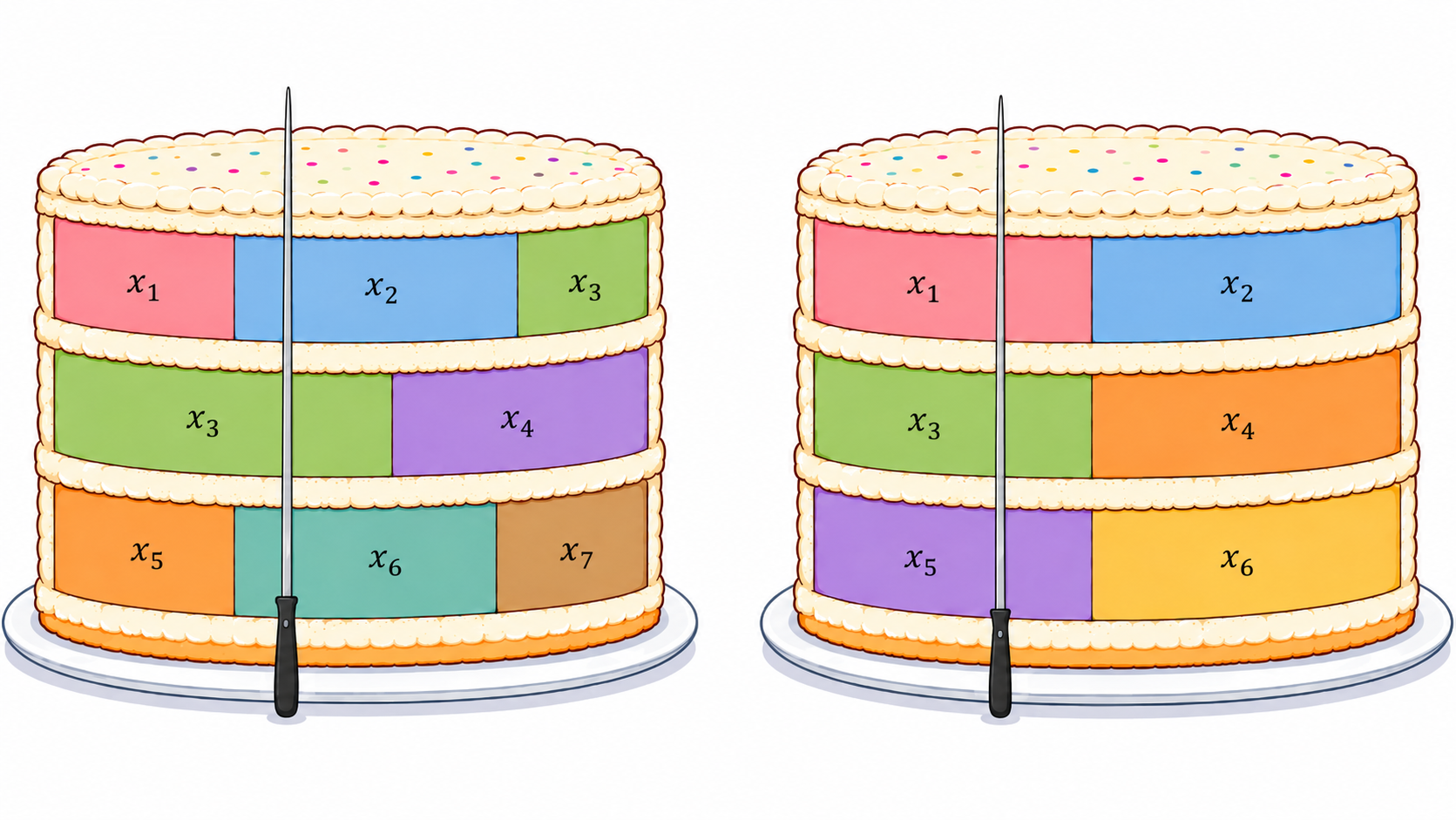
The left part of the picture above illustrates the cake-cutting process. It is clear that the \(i\)-th piece is touched by the knife with probability exactly \(x_i\), each piece is touched by the knife at most once, and exactly \(k\) pieces are touched because the knife touches each layer exactly once. Therefore (P1) and (P2) are satisfied.
However, the right part of the picture shows that the process cannot guarantee negative correlation. Suppose \(n=6\) and every piece has length \(0.5\). Then there are two equal-size pieces on each layer, and no matter where the knife cuts, it either touches \(\{1,3,5\}\) or \(\{2,4,6\}\). That is, the outcome is highly correlated, and (P3) is severely violated. For example, \[ \Pr[\bigwedge_{i\in \{1,3,5\}}(X_i=1)] = \frac{1}{2} > \frac{1}{8}= \prod_{i\in \{1,3,5\}}p_i ~. \]
Srinivasan’s Sampling Process
In this section we present Srinivasan’s sampling process, which simultaneously satisfies all three requirements. I will follow an alternative but equivalent description of the process due to DJR07.
The process can be viewed as a game that starts with each player \(i\) holding \(p_i\) units of chips. Then, in each round, two players \(i,j\) who currently hold a non-integral amount of chips are chosen to play a match. Suppose \(i\) has \(\alpha\) units of chips and \(j\) has \(\beta\) units of chips.
- If \(\alpha+\beta<1\), it is called a “bad match”. The outcome is randomized and determined independently from other matches: \(i\) wins with probability \(\frac{\alpha}{\alpha+\beta}\), and \(j\) wins with probability \(\frac{\beta}{\alpha+\beta}\). The winner takes all the chips from the loser (so now it has \(\alpha+\beta\) units of chips) and stays in the game; the loser loses all its chips and is eliminated, and we set \(X_{loser}=0\).
- If \(\alpha+\beta\geq 1\), it is called a “good match”. \(i\) wins with probability \(\frac{1-\beta}{2-\alpha-\beta}\) and \(j\) wins with probability \(\frac{1-\alpha}{2-\alpha-\beta}\). The winner grabs chips from the loser until it has \(1\) unit of chips, then it is allocated a prize (set \(X_{winner}=1\)) and leaves the game; the loser is left with \(\alpha+\beta-1\) units of chips and stays in the game. In the corner case \(\alpha+\beta=1\), the loser has \(0\) unit of chips left and is also eliminated.
The process terminates when every player is either eliminated or is allocated a prize.
In each round, the two players can be chosen arbitrarily, and next we prove that regardless of how they are chosen, the process satisfies (P1), (P2), and (P3).
Proof of (P2)
(P2) follows almost directly from the definition of the process: initially, the players hold a total of \(\sum_{i=1}^n p_i = k\) units of chips, and in each round some chips are moved from one player to the other, so in the end there are still \(k\) units of chips. Eventaully each player either holds \(1\) unit of chips and is allocated the prize, or holds \(0\) unit of chips and is eliminated, so exactly \(k\) players get the prize.
Proof of (P1)
Consider any round that involves \(i\) with \(\alpha\) chips and \(j\) with \(\beta\) chips. Let’s calculate how much the amount of chips of \(i\) changes in expectation.
If it is a bad match: \(i\) wins with probability \(\frac{\alpha}{\alpha+\beta}\) and grabs \(\beta\) chips from \(j\), otherwise it loses \(\alpha\) chips to \(j\). Therefore in expectation, \(i\)’s amount of chips changes by \[ \frac{\alpha}{\alpha+\beta}\cdot \beta + \frac{\beta}{\alpha+\beta}\cdot (-\alpha) = 0 ~. \]
If it is a good match: \(i\) wins with probability \(\frac{1-\beta}{2-\alpha-\beta}\) and grabs \(1-\alpha\) chips from \(j\), otherwise it loses \(1-\beta\) chips to \(j\). Therefore in expectation, \(i\)’s amount of chips changes by \[ \frac{1-\beta}{2-\alpha-\beta}\cdot (1-\alpha) + \frac{1-\alpha}{2-\alpha-\beta}\cdot (-1+\beta) = 0 ~. \]
Therefore, in any round that involves \(i\), the expected amount of chips that \(i\) holds does not change. This also holds obviously if a round does not involve \(i\).
So we can conclude by induction that, after any round, the expected amount of chips that \(i\) holds is \(p_i\). This means when the process terminates, \(i\) holds \(1\) unit of chips and gets a prize with probability \(p_i\).
Proof of (P3)
We only prove the first inequality \[ \Pr[\bigwedge_{i\in S}(X_i=0)] \leq \prod_{i\in S}(1-p_i) ~, \tag{1} \] the second is symmetric (by flipping \(0/1\)).
The process has an elegant inductive structure:
- If the first match is a bad match, it eliminates one player, and the remaining players still hold a total of \(k\) chips.
- If the first match is a good match, the winner gets a prize and takes \(1\) unit of chips away from the game, leaving the remaining players holding a total of \(k-1\) chips and competing for \(k-1\) prizes.
Therefore, each match effectively reduces to another instance with strictly fewer players. So we prove (P3) by induction on \(n\).
Suppose in the first round we pick two players \(i,j\), note that now \(i\) has \(p_i\) chips and \(j\) has \(p_j\) chips. We fix \(S\) and distinguish between three cases:
\(|S\cap \{i,j\}|=2\): if \(p_i+p_j\geq 1\), then at least one of \(i,j\) gets the prize , and LHS of (1) would be \(0\). Now assume \(p_i+p_j<1\), then LHS of (1) decomposes to two events: either \(i\) or \(j\) is eliminated at the first step, and the other player is eliminated later.
With probability \(\frac{p_i}{p_i+p_j}\), \(j\) is eliminated, then \(i\) has \(p_i+p_j\) chips, and by the inductive hypothesis on the resulting instance, the probability that \(i\) and the other members of \(S\) are all eliminated later is at most \[ (1-p_i-p_j)\prod_{t\in S\setminus \{i,j\}}(1-p_t) ~. \] The other event that \(i\) is eliminated is similar. So we conclude that \[ \begin{aligned} LHS \leq &~ \frac{p_i}{p_i+p_j}\cdot (1-p_i-p_j)\prod_{t\in S\setminus \{i,j\}}(1-p_t)\\ + &~ \frac{p_j}{p_i+p_j}\cdot (1-p_i-p_j)\prod_{t\in S\setminus \{i,j\}}(1-p_t)\\ = &~ (1-p_i-p_j)\prod_{t\in S\setminus \{i,j\}}(1-p_t)\\ \leq &~ (1-p_i)(1-p_j)\prod_{t\in S\setminus \{i,j\}}(1-p_t) = RHS ~. \end{aligned} \]
\(|S\cap \{i,j\}|=1\): WLOG assume \(i\in S,j\not\in S\). If the first round is a bad match, then \(i\) is eliminated with probability \(\frac{p_j}{p_i+p_j}\), otherwise \(j\) is eliminated and the game is reduced to \(i\) having \(p_i+p_j\) chips. By a similar inductive analysis, \[ \begin{aligned} LHS \leq &~ \frac{p_j}{p_i+p_j}\cdot \prod_{t\in S\setminus \{i\}}(1-p_t) + \frac{p_i}{p_i+p_j}\cdot (1-p_i-p_j)\prod_{t\in S\setminus \{i\}}(1-p_t)\\ = &~ (1-p_i)\prod_{t\in S\setminus \{i\}}(1-p_t) = RHS ~. \end{aligned} \] If the first round is a good match, then with probability \(\frac{1-p_i}{2-p_i-p_j}\), \(i\) stays in the match with \(p_i+p_j-1\) chips, otherwise it gets the prize. Therefore \[ \begin{aligned} LHS \leq &~ \frac{1-p_i}{2-p_i-p_j}\cdot (1-(p_i+p_j-1))\prod_{t\in S\setminus \{i\}}(1-p_t)\\ = &~ (1-p_i)\prod_{t\in S\setminus \{i\}}(1-p_t) = RHS ~. \end{aligned} \]
\(|S\cap \{i,j\}|=0\): whatever happens at this step, the inductive hypothesis implies that the resulting subproblem guarantees (1) for \(S\).
References
- [Sri01] Srinivasan, A. (2001). Distributions on Level-Sets with Applications to Approximation Algorithms.
- [GKPS06] Gandhi, R., Khuller, S., Parthasarathy, S., and Srinivasan, A. (2006). Dependent Rounding and Its Applications to Approximation Algorithms.
- [DJR07] Dubhashi, D. P., Jonasson, J., and Ranjan, D. (2007). Positive Influence and Negative Dependence.
- [BSS18] Byrka, J., Skowron, P., and Sornat, K. (2018). Proportional Approval Voting, Harmonic \(k\)-Median, and Negative Association.
- [NSW25] Naor, J., Srinivasan, A., and Wajc, D. (2025). Online Dependent Rounding Schemes for Bipartite Matchings, with Applications.
Comments